Voronoi tessellation and plotting functionality
With all of the effort but into building a instrument acquiring as much data and data points as possible, it is sensible to have a plotting algorithm that then shows all of these. This is exactly what the two methods plotA3A4 and plotQPatches seek to do. However, performing calculations and plotting all of the measured points make the methods computationally heavy and slow as well as presents challenges for the visualization. Below is a list of difficulties encountered while building the two methods.
Difficulties:
Handle (almost) duplicate point positions
Generate suitable patch around all points
Number of points to handle
The methods do address some of the above challenges in some way; the almost duplicate points are handled by truncating the precision on the floating point values holding the position. That is, \(\vec{q}=\left(0.1423,2.1132\right)\) is by default rounded to \(\vec{q}=\left(0.142,2.113\right)\) and binned with other points at the same position. This rounding is highly relevant when generating patches in \(A3\)-\(A4\) coordinates as the discretization is intrinsic to the measurement scans performed.
What is of real interest is the generation of a suitable patch work around all of the points for which this page is dedicated. The wanted method is to be agile and robust to be able to handle all of the different scenarios encountered. For these requirements to be met, the voronoi tessellation has been chosen.
Voronoi tessellation
First of all, the voronoi diagram is defined as the splitting of a given space into regions, where all points in one region is closer to one point than to any other point. That is, given an initial list of points, the voronoi algorithm splits of space into just as many regions for which all points in a given region is closest to the initial point inside it than to any other. This method is suitable in many different areas of data treatment, e.g. to divide a city map in to districts depending on which hospital is nearest. This method can however also be used in the specific task for creating pixels around each measurement point in a neutron scattering dataset.
The method works in n-dimensional spaces, where hyper-volumes are created, and one can also change the distance metric from the normal Euclidean \(d = \sqrt{\Delta x^2+\Delta y^2+\Delta z^2 \cdots}\) to other metrics, i.e. the so-called Manhattan distance \(d = |\Delta x|+|\Delta y|+|\Delta z|+\cdots\). It has, however, been chosen that using multi-dimensional and non-Euclidean tessellations obscures the visualization of the data rather than enhancing it. Furthermore, the used SciPi-package spatial does not natively support changes of metric and a rewriting is far outside of the scope of this software suite.
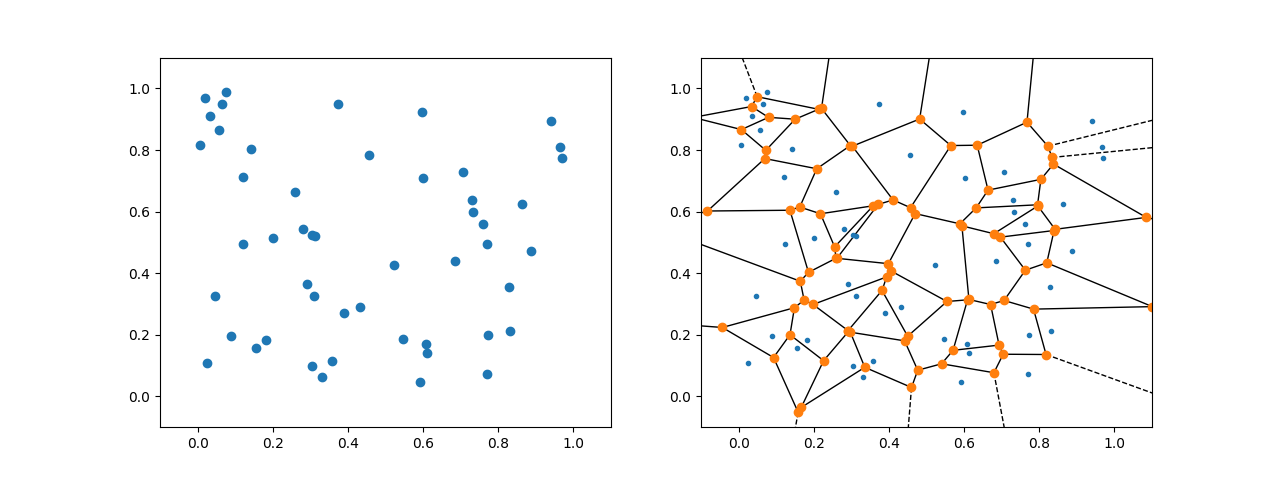
Left: 50 random points generated and plotted in 2D. Right: Voronoi diagram created for the 50 random points. Blue points are initial positions, orange are intersections, full lines are edges (denoted ridges) connecting two intersections, dashed lines go to infinity.
As seen above, for a random generated set of points, the voronoi tessellation is also going to produce a somewhat random set of edges. This is of course different, if instead one had a structured set of points as in StructuredVoronoi below. However, some of the edges still go to infinity creating infinitely large pixels for all of the outer measurements. This is trivially un-physical and is to be dealt with by cutting or in another way limiting the outer pixels.
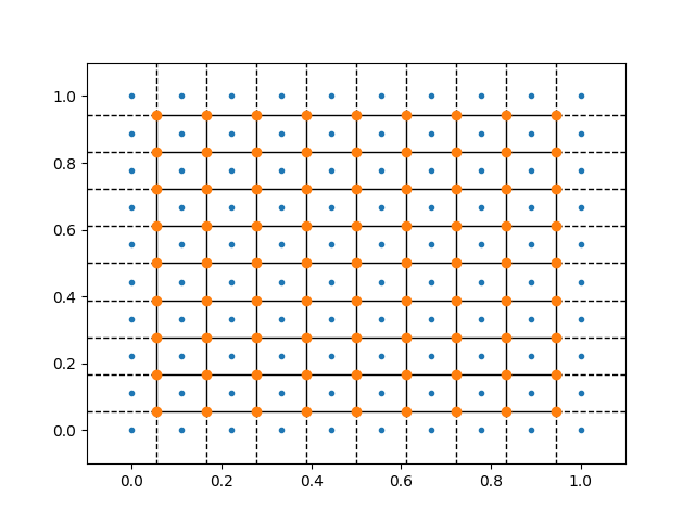
Voronoi generated for regular set of data points as for instance an \(A3\) rotation scan with equidistant \(A4\) points.
From the above, it is even more clear that the edge pixels extend to infinity. This is to be taken care of and two ways comes into mind. First, one could define a boundary such that the pixel edges intersecting this boundary is cut in a suitable manor. Second, one could add an extra set of data points around the actual measurement points in such a way that all of the wanted pixels remain finite. Both of these methods sort of deals with the issue but ends up also creating more; when cutting the boundary it still remains to figure out how and where the infinite lines intersect with it and how to best cut; adding more points is in principle simple but how to choose these suitably in all case. In the reality a combination of the two is what is used. That is, first extra points are added all around the measurement area, generating a bigger voronoi diagram; secondly the outer pixels are cut by the boundary. Thus the requirement on the position of the additional points is loosened as one is free to only add a small amount of extra points (specifically 8 extra points are added: above, below, left, right, and diagonally, with respect to the mean position).