Constant Energy Q-plane

After one has gotten an overview of the data measured through the Viewer3D (explained in QuickView3D.html the next step is to plot only as single plane of constant energy as function of H, K, and L or \(Q_x\) and \(Q_y\) and depending on the boolean state of the “rlu” key word argument. Two different binning methods are currently provided: Polar and XY. What is done is that the points measured are binned either. For explanation of units and size of bins, see below

%matplotlib inline


from MJOLNIR.Data import DataSet
from MJOLNIR import _tools # Usefull tools useful across MJOLNIR
import numpy as np
import matplotlib.pyplot as plt

Next, loading of the data files and converting using binning 8

numbers = '483-489,494-500' # String of data numbers
fileList = _tools.fileListGenerator(numbers,r'C:\Users\lass_j\Documents\CAMEA2018',2018) # Create file list from 2018 in specified folder


# Create the data set
ds = DataSet.DataSet(fileList)
ds.convertDataFile(binning=8)

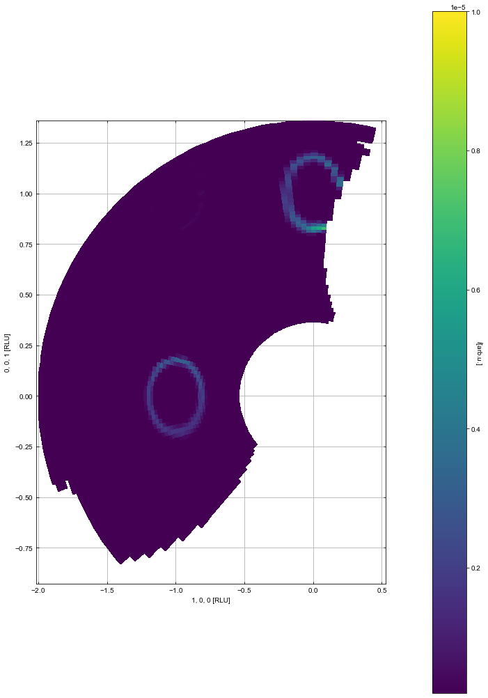
Setting up the constant energy cut, one needs to provide the energy range over which the data are integrated as well as the size of the pixels. First example utilizes polar binning where x corresponds to the radial direction and y the tangental, i.e. angular, direction.

%matplotlib inline
# Choose energy limits for binning
EMin = 3.5
EMax = 4.0
# Generate a figure making use of binning in polar coordinates
Data,ax = ds.plotQPlane(EMin=EMin, EMax=EMax,xBinTolerance=0.03,yBinTolerance=0.03,
                        binning='polar',vmin=2e-7,vmax=1e-5, colorbar= True)

#The above figure is a bit too far zoomed out. Luckily, the axis has a method to zoom to include a given RLU point
ax.set_xlim(-2.6,0.68)
ax.set_ylim(-1.76,2.58)
ax.get_figure().set_size_inches(12,18)

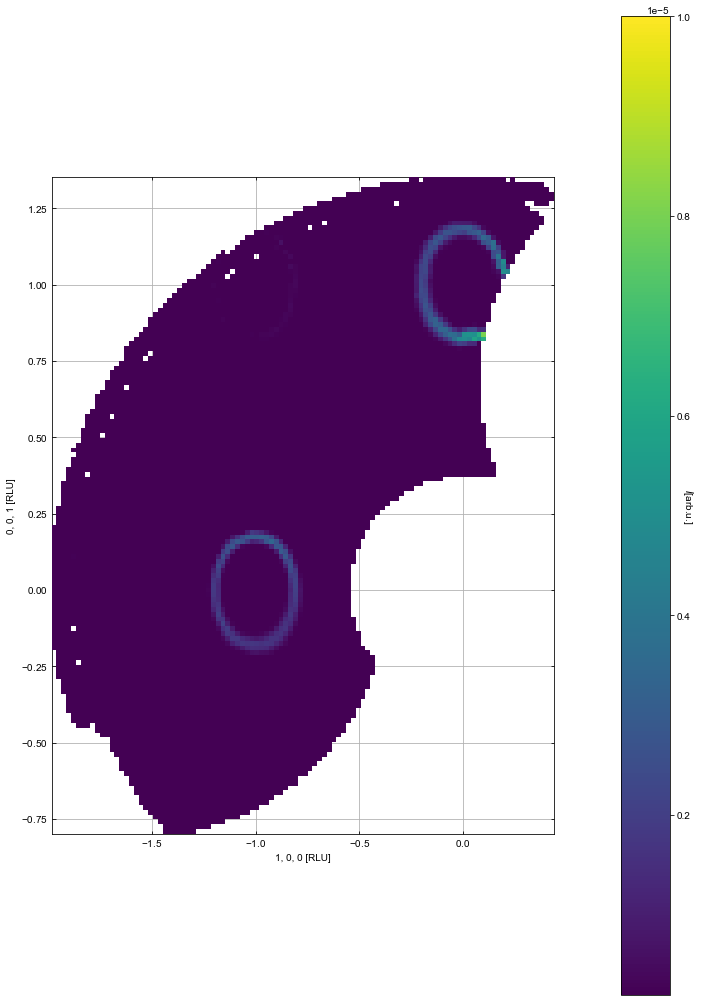
Next, generating the same figure as above but utilizing pixels as defined in \(Q_x\) and \(Q_y\)

%matplotlib inline
Data2,ax2 =  ds.plotQPlane(EMin=EMin, EMax=EMax,xBinTolerance=0.03,yBinTolerance=0.03,
                           binning='xy',vmin=2e-7,vmax=1e-5,colorbar=True)

ax2.get_figure().set_size_inches(12,18)

Binnings explained

The bin sizes depends on the other parameters provided to the method. The tables below seeks to show all of the possibilities:

Binning (rlu=False)	Parameter	Unit	Limits	Comment
XY	xBinTolerance	1/AA	(0,:math:infty)	Binning along \(Q_x\)
XY	yBinTolerance	1/AA	(0,:math:infty)	Binning along \(Q_y\)
Ploar	xBinTolerance	rad	(0,2:math:pi]	Angular Binning
Ploar	yBinTolerance	1/AA	(0,:math:infty)	Radial Binning

With rlu true

Binning (rlu=True)	Parameter	Unit	Limits	Comment
XY	xBinTolerance	RLU	(0,:math:infty)	Binning along first projection vector
XY	yBinTolerance	RLU	(0,:math:infty)	Binning along second projection vector
Ploar	xBinTolerance	rad	(0,2:math:pi]	Angular Binning
Ploar	yBinTolerance	RLU	(0,:math:infty)	Radial Binning

For further explanation of the RLU axis see Reciprocal Lattice Unit Axis